Figure.add_subplot()メソッドで projection に “3d” を渡すと、3次元データを可視化するためのサブプロット (mpl_toolkits.mplot3d.Axes3Dクラスのインスタンス) が追加されます。Axes3Dオブジェクトには以下のようなメソッドが備わっています。
・Axes3D.plot() パラメータ曲線
・Axes3D.plot_surface() 曲面
・Axes3D.plot_surface() 平面と法線
・Axes3D.scatter() 散布図
・Axes3D.plot_wireframe() ワイヤーフレーム
・Axes3D.plot_trisurf() パラメータ曲面
・Axes3D.contour() 3次元等高線
・Axes3D.init_view() 視点の変更
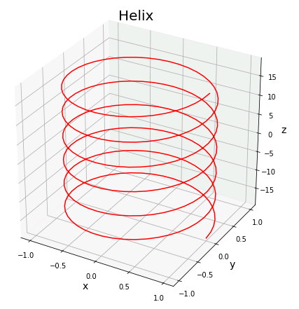
パラメータ曲線
Axes3D.plot() を使うと、パラメータ $t$ で媒介される空間曲線
\[x=x(t),\ y=y(t),\ z=z(t)\]
を描くことができます。
Axes3D.plot(xs, ys, *args, **kwargs)
引数 xs, ys には曲線の (x, y) 座標を渡します。3 つめの引数を記述すると、z 座標 zs が指定されたことになります。キーワード引数で線の種類や色などを選択することもできます。zdir引数では、縦軸にとる変数を選ぶことができます (デフォルトは z です)。以下のサンプルコードでは
\[x=\cos t,\quad y=\sin t,\quad z=t\]
という方程式で表される螺旋(らせん)を描いてみます。
# PYTHON_MATPLOTLIB_3D_PLOT_01

import numpy as np
import matplotlib.pyplot as plt
from mpl_toolkits.mplot3d import Axes3D

# Figureを追加
fig = plt.figure(figsize = (8, 8))

# 3DAxesを追加
ax = fig.add_subplot(111, projection='3d')

# Axesのタイトルを設定
ax.set_title("Helix", size = 20)

# 軸ラベルを設定
ax.set_xlabel("x", size = 14)
ax.set_ylabel("y", size = 14)
ax.set_zlabel("z", size = 14)

# 軸目盛を設定
ax.set_xticks([-1.0, -0.5, 0.0, 0.5, 1.0])
ax.set_yticks([-1.0, -0.5, 0.0, 0.5, 1.0])

# 円周率の定義
pi = np.pi

# パラメータ分割数
n = 256

# パラメータtを作成
t = np.linspace(-6*pi, 6*pi, n)

# らせんの方程式
x = np.cos(t)
y = np.sin(t)
z = t

# 曲線を描画
ax.plot(x, y, z, color = "red")

plt.show()
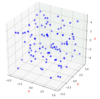
3次元散布図
Axes3D.scatter() は 3 次元散布図を描くメソッドです。
Axes3D.scatter(xs, ys, zs=0, zdir='z',
s=20, c=None, depthshade=True, *args, **kwargs)
xs, ys は各点の x 座標と y 座標です。
zs は z 座標です。デフォルトでは 0 に設定されています。
zdir は縦軸にとる変数です。
s はマーカーの大きさ、c はマーカーの色です。
depthshade はマーカーに影をつけるオプションです。
以下のサンプルコードでは、numpy.random.rand() を使って、3 次元座標にランダムな点をプロットします。
# PYTHON_MATPLOTLIB_3D_PLOT_02

# 3次元散布図

import numpy as np
import matplotlib.pyplot as plt
from mpl_toolkits.mplot3d import Axes3D

# Figureを追加
fig = plt.figure(figsize = (8, 8))

# 3DAxesを追加
ax = fig.add_subplot(111, projection='3d')

# Axesのタイトルを設定
ax.set_title("", size = 20)

# 軸ラベルを設定
ax.set_xlabel("x", size = 14, color = "r")
ax.set_ylabel("y", size = 14, color = "r")
ax.set_zlabel("z", size = 14, color = "r")

# 軸目盛を設定
ax.set_xticks([-5.0, -2.5, 0.0, 2.5, 5.0])
ax.set_yticks([-5.0, -2.5, 0.0, 2.5, 5.0])

# -5~5の乱数配列(100要素)
x = 10 * np.random.rand(100, 1) - 5
y = 10 * np.random.rand(100, 1) - 5
z = 10 * np.random.rand(100, 1) - 5

# 曲線を描画
ax.scatter(x, y, z, s = 40, c = "blue")

plt.show()
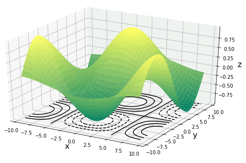
3次元等高線
Axes3D.contour() は 3 次元座標に等高線を配置するメソッドです。
Axes3D.contour(X, Y, Z, *args, **kwargs)
X, Y には 2 次元配列を与えます(一般には格子点データを作成します)。Z には各 (X, Y) に対応する高度のデータをあたえます。キーワード引数の offset で、等高線を描いた平面を設置する z 座標を指定できます。この引数を省略すると、自動で z 軸方向に等間隔に何枚かの等高線平面が重ね合わせられます。以下のサンプルコードを実行すると、2 変数関数 $z=\cos x \sin x$ の曲面と等高線を同時に描きます。
# PYTHON_MATPLOTLIB_3D_PLOT_03

import numpy as np
import matplotlib.pyplot as plt
from mpl_toolkits.mplot3d import Axes3D

# Figureと3DAxeS
fig = plt.figure(figsize = (8, 8))
ax = fig.add_subplot(111, projection="3d")

# 軸ラベルを設定
ax.set_xlabel("x", size = 16)
ax.set_ylabel("y", size = 16)
ax.set_zlabel("z", size = 16)

# 円周率の定義
pi = np.pi

# (x,y)データを作成
x = np.linspace(-3*pi, 3*pi, 256)
y = np.linspace(-3*pi, 3*pi, 256)

# 格子点を作成
X, Y = np.meshgrid(x, y)

# 高度の計算式
Z = np.cos(X/pi) * np.sin(Y/pi)

# 曲面を描画
ax.plot_surface(X, Y, Z, cmap = "summer")

# 底面に等高線を描画
ax.contour(X, Y, Z, colors = "black", offset = -1)

plt.show()