ガンマ関数
整数 $n$ について階乗 $n!$ は
\[n!=\begin{cases}1 & (n=0)\\[6pt]n(n-1)(n-2)\ \cdots\ 2\cdot 1 & (n\geq 1)\end{cases}\]
によって定義されますが、$n$ を実部が正となる複素数 $z$ にまで拡大定義した連続関数をガンマ関数とよびます。
\[\Gamma(z)=\int_{0}^{\infty} e^{-t}t^{z-1}\tag{1}dt\]
$z$ が整数 $n$ であるとき、ガンマ関数と階乗の間には次のような関係があります。
\[\Gamma(n+1)=n!\tag{2}\]
$z$ が非整数であっても、$\Gamma(z)$ は以下の公式によって再帰計算することができます。
\[\Gamma(z+1)=z\Gamma(z)\tag{3}\]
また、$z=1/2$ におけるガンマ関数の値を (1) によって計算すると
\[\Gamma \left( \frac{1}{2}\right)=\sqrt{\pi}\tag{4}\]
となり、半整数値におけるガンマ関数の値は
\[\Gamma \left( n+\frac{1}{2}\right) =\frac{(2n-1)!!}{2^n}\sqrt{\pi} \tag{5}\]
で表せることが知られています。
math.gamma(x) を使って、正数 x におけるガンマ関数の値を計算できます。
# GAMMA_FUNCTION

# In[1]

from math import gamma

# Γ(4)=3!
val = gamma(4)

print(val)
# 6.0
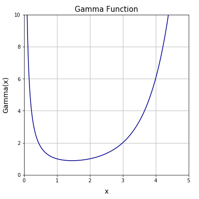
Matplotlib を使って、ガンマ関数をグラフに描いてみます。ただし、NumPy にはガンマ関数を計算する関数が用意されていないので、frompyfunc() を使って、math.gamma() をユニバーサル関数に変換しておきます。
# In[2]

import numpy as np
import matplotlib.pyplot as plt

# x座標データを作成
x = np.linspace(0.01, 5, 257)

# math.gamma()をユニバーサル化
gamma_u = np.frompyfunc(gamma, 1, 1)

# y座標データを作成
y = gamma_u(x)

# ガンマ関数のグラフを描画
fig = plt.figure(figsize = (6, 6))
ax = fig.add_subplot(111)
ax.set_title("Gamma Function", size = 15)
ax.grid()
ax.set_xlim(0, 5)
ax.set_ylim(0, 10)
ax.set_xlabel("x", size = 14, labelpad = 10)
ax.set_ylabel("Gamma(x)", size = 14, labelpad = 10)
ax.plot(x, y, color = "darkblue")
math.lgamma(x) はガンマ関数の自然対数を返します。
# In[3]

# log{Γ(3.5)}
val = lgamma(3.5)

print("{:3.f}".format(val))
# 1.201
SciPy の special.gamma(z) は任意の複素数 z を受け取ってガンマ関数の値を返します。
# In[4]

from scipy.special import gamma

# Γ(2+3i)
val = gamma(2 + 3j)

print("{:.3f}".format(val))
# -0.082+0.092j
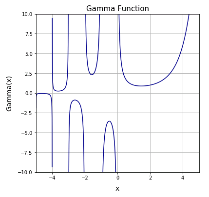
Matplotlib を使って、全実数領域におけるガンマ関数の値をグラフにプロットしてみます。
# In[5]

# x座標データを作成
x = np.linspace(-5, 5, 2251)

# y座標データを作成
y = gamma(x)

# ガンマ関数のグラフを描画
fig = plt.figure(figsize = (6, 6))
ax = fig.add_subplot(111)
ax.set_title("Gamma Function", size = 15)
ax.grid()
ax.set_xlim(-5, 5)
ax.set_ylim(-10, 10)
ax.set_xlabel("x", size = 14, labelpad = 10)
ax.set_ylabel("Gamma(x)", size = 14, labelpad = 10)
ax.plot(x, y, color = "darkblue")
plt.show()
scipy.special.gammaln() はガンマ関数の自然対数を高精度で計算します。
# In[6]

from scipy.special import gammaln

# logΓ(10)
val = gammaln(10)

print("{:.3f}".format(val))
# 12.802
ディガンマ関数
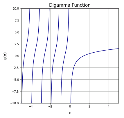
ガンマ関数の対数微分をディガンマ関数とよびます。
\[\psi(z)=\frac{d}{dz}\ln\Gamma(z)\tag{6}\]
SciPy にはディガンマ関数を計算する scipy.special.psi(x) が用意されています。
# DIGAMMA_FUNCTION

# In[1]

from scipy.special import psi

# ψ(-1.5),ψ(1),ψ(2)
val = psi(-1.5)

print("{:.3f}".format(val))
# 0.423
$\gamma=-\psi(1)$ はオイラーの定数とよばれます。
# In[2]

# オイラーの定数
g = -psi(1)

print("γ = {}".format(g))
# γ = 0.5772156649015329
オイラーの定数は numpy.euler_gamma で呼び出すこともできます。
# In[3]

import numpy as np

# NumPyのオイラー定数
g = np.euler_gamma

print("γ = {}".format(g))
# 0.5772156649015329
ディガンマ関数には
\[\psi(x+1)=\psi(x)+\frac{1}{x}\tag{7}\]
という性質があるので、整数点におけるディガンマ関数は有限調和級数からオイラーの定数を差し引いた形で表されます。
\[\psi(n+1)=1+\frac{1}{2}+\frac{1}{3}+\ \cdots \ +\frac{1}{n}-\gamma\tag{8}\]
実数範囲でディガンマ関数をプロットするコードを載せておきます。
# In[4]

import matplotlib.pyplot as plt

# x座標データを作成
x = np.linspace(-5, 5, 2251)

# y座標データを作成
y = psi(x)

# ディガンマ関数のグラフを描画
fig = plt.figure(figsize = (6, 6))
ax = fig.add_subplot(111)
ax.set_title("Digamma Function", size = 15)
ax.grid()
ax.set_xlim(-5, 5)
ax.set_ylim(-10, 10)
ax.set_xlabel("x", size = 14, labelpad = 10)
ax.set_ylabel("ψ(x)", size = 14, labelpad = 10)
ax.plot(x, y, color = "darkblue")
ポリガンマ関数
ディガンマ関数 $\psi(z)$ の $1$ 階微分 $\psi^{(1)}(z)$、$2$ 階微分 $\psi^{(2)}(z)$、$3$ 階微分 $\psi^{(3)}(z)$ … をそれぞれトリガンマ関数、テトラガンマ関数、ペンタガンマ関数 … とよび、これらの総称をポリガンマ関数 $\psi^{(n)}(z)$ と定義します。
\[\psi^{(n)}=\frac{d^{n+1}}{dz^{n+1}}\ln\Gamma(z)\tag{9}\]
SciPy にはポリガンマ関数を計算する scipy.special.polygamma(n,x) が用意されています。
# POLYGAMMA__FUNCTION

# In[1]

from scipy.special import polygamma

# z=1におけるディガンマ関数の値
di = polygamma(0, 1)

# z=1におけるトリガンマ関数の値
tri = polygamma(1, 1)

# z=1におけるテトラガンマ関数の値
tetra = polygamma(2, 1)

print("ψ(1): {:.3f}".format(a))
print("ψ1(1): {:.3f}".format(b))
print("ψ2(1): {:.3f}".format(c))

# ψ(1): -0.577
# ψ1(1): 1.645
# ψ2(1): -2.404
不完全ガンマ関数
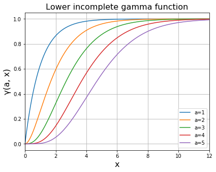
ガンマ関数の積分区間 $[0,\infty]$ を 2 つに分割して、不完全ガンマ関数を次のように定義します。
\[\begin{align*}\gamma(a,x)&=\int_0^xe^{-t}t^{a-1}\tag{10}\\[6pt]\Gamma(a,x)&=\int_x^{\infty}e^{-t}t^{a-1}=\Gamma(a)-\gamma(a,x)\tag{11}\end{align*}\]
(10) を第1種不完全ガンマ関数 (lower incomplete gamma function)、(11) を第2種不完全ガンマ関数 (upper incomplete gamma function) とよびます。
scipy.special.gammainc(a,x) は第1種不完全ガンマ関数 $\gamma(a,x)$ を計算します。
INCOMPLETE_GAMMA_FUNCTION

# In[1]

import numpy as np
from scipy.special import gammainc
import matplotlib.pyplot as plt

# 区間[0,12]を128分割
x = np.linspace(0, 12, 129)

# FigureとAxes
fig = plt.figure(figsize=(6.5, 5))
ax = fig.add_subplot(111)
ax.grid()
ax.set_title("Lower incomplete gamma function", fontsize=16)
ax.set_xlabel("x", fontsize=16)
ax.set_ylabel("γ(a, x)", fontsize=16)
ax.set_xlim(0, 12)
#ax.set_ylim(0, 10)

# 第1種不完全ガンマ関数をプロット
for a in range(1, 6):
    ax.plot(x, gammainc(a, x), label="a={}".format(a))

# 凡例を表示
ax.legend(loc="lower right")
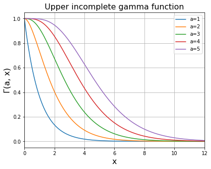
scipy.special.gammaincc(a,x) は第2種不完全ガンマ関数 $\Gamma(a,x)$ を計算します。
# In[2:

# 区間[0,12]を128分割
x = np.linspace(0, 12, 129)

# FigureとAxes
fig = plt.figure(figsize=(6.5, 5))
ax = fig.add_subplot(111)
ax.grid()
ax.set_title("Upper incomplete gamma function", fontsize=16)
ax.set_xlabel("x", fontsize=16)
ax.set_ylabel("Γ(a, x)", fontsize=16)
ax.set_xlim(0, 12)
#ax.set_ylim(0, 10)

# 第2種不完全ガンマ関数をプロット
for a in range(1, 6):
    ax.plot(x, gammaincc(a, x), label="a={}".format(a))

# 凡例を表示
ax.legend(loc="upper right")
コメント