ルジャンドル多項式
ルジャンドルの微分方程式
\[\frac{d}{dx}\left[(1-x^2)\frac{df(x)}{dx}\right]+n(n+1)f(x)=0\tag{1}\]
の解 $P_n(x)$ を ルジャンドル多項式 (Legendre polynomial) とよび、
\[P_0(x),\ P_1(x),\ P_2(x),\ P_3(x),\ …\]
は区間 [$-1,\ 1$] で直交関数系をなします:
\[\int_{-1}^{1}P_m(x)P_n(x)dx=\frac{2}{2n+1}\delta_{mn}\tag{2}\]
$P_n(x)$ は漸化式
\[\begin{align*}&P_0(x)=1\\[6pt]&P_1(x)=x\\[6pt]&(n+1)P_{n+1}(x)=(2n+1)xP_n(x)-nP_{n-1}(x)\end{align*}\tag{3}\]
から逐次生成することができます。具体的表式を並べると以下のようになります。
\[\begin{align*}&P_0(x)=1\\[6pt]&P_1(x)=x\\[6pt]&P_2(x)=\frac{1}{2}(x^2-1)\\[6pt]&P_3(x)=\frac{1}{2}(x^3-3x)\\[6pt]&P_4(x)=\frac{1}{8}(x^4-30x^2+3)\end{align*}\]
ルジャンドル多項式はロドリゲスの公式
\[P_n(x)=\frac{1}{2^nn!}\frac{d^n}{dx^n}(x^2-1)^n\tag{4}\]
から求めることもできます。
scipy.special.eval_legendre()
scipy.special.eval_legendre(n, x) は n 次のルジャンドル多項式の点 x における値を評価します。
# PYTHON_LEGENDRE_POLYNOMIAL

# In[1]

x = np.linspace(-1, 1, 5)

# 4次のルジャンドル多項式のxにおける値を計算
p = eval_legendre(4, x)

print(p)
# [ 1.        -0.2890625  0.375     -0.2890625  1.       ]
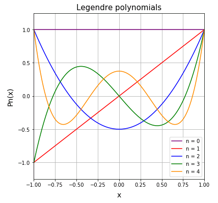
以下のコードを実行すると、ルジャンドル多項式のグラフを描画します。
# In[2]

# FigureとAxesを設定
fig = plt.figure(figsize = (6, 6))
ax = fig.add_subplot(111)
ax.set_title("Legendre polynomials", size = 15)
ax.grid()
ax.set_xlim(-1, 1)
ax.set_ylim(-1.25, 1.25)
ax.set_xlabel("x", size = 14, labelpad = 8)
ax.set_ylabel("Pn(x)", size = 14, labelpad = 8)

# x座標データ
x = np.linspace(-1, 1, 129)

# 色のリスト
c = ["red", "blue", "green", "darkorange", "purple"]

# P0,P1,P2,P3,P4のグラフを描画
for i in range(5):
    ax.plot(x, eval_legendre(i, x),
            label = "n = {}".format(i), color = c[i-1])

# 凡例を表示
ax.legend()

plt.show()
scipy.special.legendre()
scipy.special.legendre(n) はルジャンドル多項式オブジェクトを生成します。
# SCIPY_SPECIAL_LEGENDRE

# In[1]

# 4次のルジャンドル多項式を生成
p4 = legendre(4)

print(p4)
#        4             3        2
# 4.375 x + 4.857e-16 x - 3.75 x + 2.429e-16 x + 0.375
多項式オブジェクトを積分する integ()メソッドを使って、$P_3(x)P_5(x)$ の [$-1,\ 1$] にわたる積分が $0$ になることを確認してみます。
# In[2]

# 3次のルジャンドル多項式
p3 = legendre(3)

# 5次のルジャンドル多項式
p5 = legendre(5)

# p3*p5の不定積分
p3p5_i = (p3 * p5).integ()

# p3*p5の[-1,1]にわたる積分
p3p5_id = p3p5_i(1)-p3p5_i(-1)

print(p3p5_id)
# 1.1102230246251565e-15
近似計算なので若干の誤差はありますが、ほぼ $0$ になっています。
ルジャンドル陪関数
ルジャンドルの陪微分方程式
\[\left[(1-x^2)\frac{d^2}{dx^2}-2x\frac{d}{dx}+n(n+1)-\frac{m^2}{1-x^2}\right]f(x)=0\tag{5}\]
の解を ルジャンドル陪関数 (Associated Legendre polynomials) とよびます:
\[P_n^{m}(x)=\frac{1}{2^mm!}(1-x^2)^{m/2}\frac{d^{m+n}}{dx^{m+n}}(x^2-1)^n\tag{6}\]
右辺の $(x^2-1)^n$ が $2n$ 次多項式なので、$2n+1$ 回の微分で $0$ になります。
したがって、ルジャンドル陪関数は
\[-n\leq m\leq n\]
の範囲で意味をもちます。いくつかの $n$ と $m$ について $P_n^{m}(x)$ を書き並べてみます。
\[\begin{align*}&P_0^{0}(x)=1\\[6pt]&P_1^{0}(x)=x\\[6pt]&P_1^{1}(x)=\sqrt{1-x^2}\\[6pt]&P_2^{0}(x)=\frac{1}{2}(3x^2-1)\\[6pt]&P_2^{1}(x)=3x\sqrt{1-x^2}\\[6pt]&P_2^{2}(x)=3(1-x^2)\end{align*}\]
scipy.special.lpmv()
scipy.special.lpmv(x1, x2, x3) はルジャンドル陪関数の値を返します。
引数を (6) の表式に合わせると lpmv(m, n, x) です。
# PYTHON_ASSOCIATED_LEGENDRE

# In[1]

# P(m=1,n=2,x=0.5)を計算
p = lpmv(1,2,0.5)

print(p)
# -1.299038105676658
すべての引数に配列を渡すことができます。たとえば、$m=0,\ x=0.5$ に固定して、$P_{0}^{0}(0.5),\ P_{1}^{0}(0.5),\ P_{2}^{0}(0.5)$ をまとめて計算させることができます。
# In[2]

n = [0, 1, 2]
p = lpmv(0, n, 0.5)

print(p)
# [ 1.     0.5   -0.125]
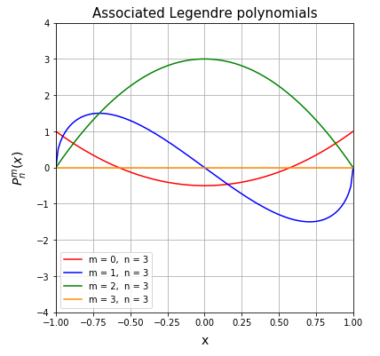
以下のコードを実行すると、$P_{3}^{0}(x),\ P_{3}^{1}(x),\ P_{3}^{2}(x),\ P_{3}^{3}(x)$ のグラフをプロットします。
# In[3]
# ルジャンドル陪関数のグラフ

# FigureとAxesを設定
fig = plt.figure(figsize = (6, 6))
ax = fig.add_subplot(111)
ax.set_title("Associated Legendre polynomials", size = 15)
ax.grid()
ax.set_xlim(-1, 1)
ax.set_ylim(-4, 4)
ax.set_xlabel("x", size = 14, labelpad = 8)
ax.set_ylabel("$P_n^m(x)$", size = 14, labelpad = 8)

# x座標データ
x = np.linspace(-1, 1, 129)

# 色のリスト
c = ["red", "blue", "green", "darkorange"]

# ルジャンドル陪関数のグラフをプロット
for i in range(4):
    ax.plot(x, lpmv(i, j, x),
            label = "m = {},  n = 3".format(i), color = c[i])

# 凡例を表示
ax.legend()

plt.show()
コメント